
1.1 Coding in JAX#
JAX looks like NumPy but behaves like a compiler. Code written in JAX can be
transformed: differentiated (jax.grad), compiled for speed (jax.jit), and applied
across whole ensembles at once (jax.vmap). This chapter is organized around one
question: what breaks when you port your NumPy code to JAX, and why? Every
restriction has the same origin: for JAX to transform your code, it must be able to
treat it as a mathematical function, not as a sequence of instructions.
Outline
Explain what tracing is and why JAX requires functions to be pure
Port a small NumPy computation to JAX, fixing in-place assignment and
ifstatementsUse
jax.jit,jax.vmap, parameter dictionaries (pytrees), and explicit random keysRecognize the failure modes collected in the gotchas appendix
import jax
import jax.numpy as jnp
import matplotlib.pyplot as plt

jax.config.update("jax_enable_x64", True)   # climate work needs double precision
# Running on Colab? First run:  %pip install -q optax equinox diffrax
From NumPy to jax.numpy#
jax.numpy (imported as jnp by convention) reproduces most of NumPy. Array creation,
arithmetic, reductions, and linear algebra carry over unchanged. Here is an area-weighted
global mean of a zonal temperature profile, written identically in both libraries:
import numpy as np

lat = np.linspace(-89, 89, 90)                      # latitude, degrees
T_np = 30.0 * np.cos(np.deg2rad(lat)) - 10.0        # a made-up temperature profile, degC

weights = np.cos(np.deg2rad(lat))
print("NumPy:", np.sum(T_np * weights) / np.sum(weights))

T = jnp.asarray(T_np)
w = jnp.cos(jnp.deg2rad(jnp.asarray(lat)))
print("JAX:  ", jnp.sum(T * w) / jnp.sum(w))
NumPy: 13.560748690332739
JAX:   13.560748690332748
The first thing that breaks: assignment#
JAX arrays are immutable — they cannot be modified after creation. Assigning into an array, a habit from NumPy and Fortran alike, raises an error:
try:
    T[0] = -40.0
except TypeError as e:
    print("TypeError:", e)
TypeError: JAX arrays are immutable and do not support in-place item assignment. Instead of x[idx] = y, use x = x.at[idx].set(y) or another .at[] method: https://docs.jax.dev/en/latest/_autosummary/jax.numpy.ndarray.at.html
The replacement is the .at[...].set(...) syntax, which returns a new array with
the requested element changed:
T_updated = T.at[0].set(-40.0)
print("original :", T[0])
print("updated  :", T_updated[0])
original : -9.476427806881492
updated  : -40.0
Immutability feels wasteful, but the compiler removes the cost: inside a compiled function, an update whose input is not reused is performed in place. What immutability buys is a guarantee — no function can silently modify data another function depends on. That guarantee is what makes automatic differentiation of large programs tractable.
Pure functions and tracing#
A pure function returns outputs that depend only on its explicit inputs, and does
nothing else — no printing, no writing to globals, no modifying its arguments. JAX
requires purity because of how its transformations work: they run your function once
with abstract tracer values in place of real arrays, record every mathematical
operation encountered, and then transform the recorded computation. Anything that is
not a recorded operation — such as a print — happens once, during tracing, and never
again:
@jax.jit
def absorbed_shortwave(albedo):
    print("  (tracing now — this line runs only when JAX records the function)")
    return 340.0 * (1.0 - albedo)

print("first call: ", absorbed_shortwave(0.3))
print("second call:", absorbed_shortwave(0.32))   # no print: the recording is reused
  (tracing now — this line runs only when JAX records the function)
first call:  237.99999999999997
second call: 231.2
The first call traces and compiles; the second reuses the compiled code. This is
also why side effects inside model code silently disappear: they are not part of the
recorded mathematics. For printing inside compiled code, use jax.debug.print
(Chapter 3.5 uses it to hunt down invalid values).
jit: compile once, run fast#
jax.jit compiles a traced function to fast machine code. The difference matters most
for time-stepping loops. Below, the same 100-point diffusion model is stepped 2,000
times, first with a Python for loop (every step dispatched separately) and then with
jax.lax.scan, JAX’s loop construct, under jit:
import time

def diffuse(T):
    return T + 0.25 * (jnp.roll(T, 1) - 2 * T + jnp.roll(T, -1))

T0 = jnp.zeros(100).at[50].set(1.0)

t = time.perf_counter()
T_loop = T0
for _ in range(2000):
    T_loop = diffuse(T_loop)
T_loop.block_until_ready()
print(f"Python loop:      {time.perf_counter() - t:.3f} s")

@jax.jit
def diffuse_2000(T):
    T, _ = jax.lax.scan(lambda T, _: (diffuse(T), None), T, None, length=2000)
    return T

diffuse_2000(T0).block_until_ready()               # first call includes compilation
t = time.perf_counter()
T_scan = diffuse_2000(T0).block_until_ready()
print(f"jit + scan:       {time.perf_counter() - t:.4f} s")
print(f"same answer: {bool(jnp.allclose(T_loop, T_scan))}")
Python loop:      0.173 s
jit + scan:       0.0002 s
same answer: True
lax.scan(f, carry, xs) applies f repeatedly, threading a running state (the
carry) through the loop — exactly the structure of a time-stepping model. Every model
in this book is written as a pure single-step function passed to scan. Two practical
notes: .block_until_ready() forces the computation to finish before the timer stops
(JAX dispatches work asynchronously), and a jitted function recompiles whenever the
shapes of its inputs change, so keep array shapes fixed inside loops.
Control flow on traced values#
During tracing, an array’s values are unknown — only its shape and type are. A Python
if that branches on a value therefore cannot be recorded:
@jax.jit
def melt_amount(T):
    if T > 273.15:                 # branching on an unknown value
        return T - 273.15
    return 0.0

try:
    melt_amount(280.0)
except jax.errors.TracerBoolConversionError as e:
    print(str(e).split("\n")[0])
Attempted boolean conversion of traced array with shape bool[].
@jax.jit
def melt_amount(T):
    return jnp.where(T > 273.15, T - 273.15, 0.0)   # both branches recorded, one selected

print(melt_amount(280.0), melt_amount(260.0))
6.850000000000023 0.0
jnp.where(condition, a, b) evaluates both branches and selects elementwise — the
standard replacement for value-dependent if. For larger branches there is
jax.lax.cond, and for loops with a value-dependent length, jax.lax.while_loop.
Chapter 3.3 returns to where, because thresholds in physics have consequences for
gradients that go beyond syntax.
vmap: the ensemble loop, vanished#
jax.vmap turns a function of one input into a function of a batch of inputs, without
a Python loop and at compiled-loop speed. Here is a first taste of climate flavor: the
temperature response of a linear energy balance model to a step forcing
\(\Delta F\) is \(\Delta T(t) = (\Delta F/\lambda)\,(1 - e^{-\lambda t / C})\), where
\(\lambda\) is the climate feedback parameter. One line evaluates the whole ensemble of
feedback values:
years = jnp.linspace(0.0, 200.0, 400)
C = 8.0                                       # heat capacity, W yr m^-2 K^-1
dF = 4.0                                      # forcing, W m^-2

def response(lam):                            # lam: feedback parameter, W m^-2 K^-1
    return dF / lam * (1.0 - jnp.exp(-lam * years / C))

lams = jnp.linspace(0.8, 2.0, 7)
ensemble = jax.vmap(response)(lams)           # shape (7, 400): one row per member

for lam, curve in zip(lams, ensemble):
    plt.plot(years, curve, label=f"$\\lambda$ = {lam:.1f}")
plt.xlabel("years after step forcing")
plt.ylabel("warming (K)")
plt.legend(fontsize=8)
plt.title("One function, mapped over an ensemble with vmap")
plt.show()
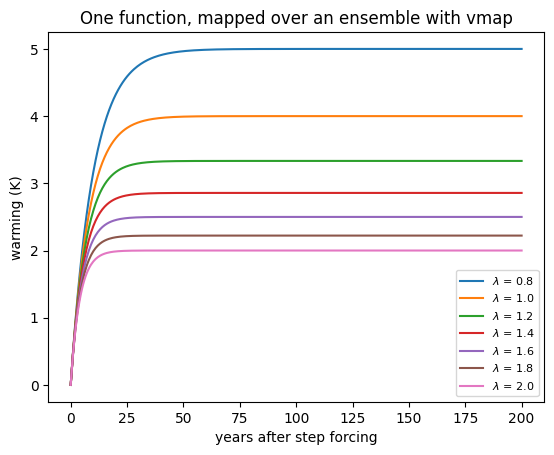
vmap composes with everything: vmap of grad gives per-member gradients,
jit of vmap compiles the whole ensemble. Chapter 2.1 uses vmap to run 60
finite-difference perturbation experiments in one call.
Pytrees: structured parameters#
Model parameters rarely live in one flat vector. JAX transformations accept pytrees — nested combinations of dictionaries, lists, and tuples with arrays at the leaves — and preserve their structure. A gradient of a function of a parameter dictionary is a dictionary of gradients with the same keys:
def outgoing_longwave(params, T):
    return params["A"] + params["B"] * T       # linearized OLR, W m^-2

params = {"A": 203.3, "B": 2.09}
dOLR = jax.grad(outgoing_longwave)(params, 15.0)
print(dOLR)      # same structure as params: sensitivity to each parameter
{'A': Array(1., dtype=float64, weak_type=True), 'B': Array(15., dtype=float64, weak_type=True)}
This is how every calibration in Part 2 is organized: physical parameters stay in a
named dictionary, and jax.grad returns the sensitivity to each one, by name.
Randomness with explicit keys#
NumPy’s random module carries hidden global state — impure by definition. JAX instead
threads randomness explicitly: a key determines a random draw completely, and
jax.random.split derives fresh, independent keys. The same key always reproduces the
same numbers, which makes ensemble experiments exactly reproducible:
key = jax.random.key(0)
key, subkey = jax.random.split(key)
perturbations = jax.random.normal(subkey, (5,))
print(perturbations)
print(jax.random.normal(subkey, (5,)))    # same key -> identical draw
[-1.4008841   1.432145    0.6248107   0.20048727  0.24714761]
[-1.4008841   1.432145    0.6248107   0.20048727  0.24714761]
Recap#
Habit from NumPy/Fortran |
JAX replacement |
|---|---|
|
|
|
|
Python |
|
|
|
|
explicit keys, |
mutating globals / arguments |
return new values; keep functions pure |
The gotchas appendix keeps the full list, including two we
enable by default throughout this book: double precision (jax_enable_x64 — JAX
defaults to single precision, which Chapter 3.5 shows is not enough for gradient
verification) and NaN debugging.
Exercises.
Write a function that sets all sub-freezing values of the profile
Tto −40 °C using.at[]with a boolean mask, then do the same withjnp.where.Use
vmapto evaluateresponseover a grid of both \(\lambda\) and \(\Delta F\) (hint: nest twovmaps).Predict what
jax.jit(lambda x: print(x) or x)(3.0)prints, then check.