3.3 Non-smooth physics

Parameterizations are full of switches. Convection triggers when instability crosses a threshold; water freezes at 0 °C; fluxes are clipped to keep quantities positive. Each switch is an if in physical clothing — and at a switch, the derivative is zero on both sides and undefined at the jump. Automatic differentiation handles such code without complaint and returns something technically correct and scientifically useless: the slope of the flat parts.

This chapter builds the failure in its purest form — a precipitation trigger — and repairs it three ways, in increasing order of sophistication: smooth the physics, reformulate the physics, or keep the physics and prescribe a better derivative.

Learning goals

• Predict what autodiff returns at where/maximum-style thresholds

• Recognize the signature of a switch-dominated loss: it varies, yet its gradient is zero

• Repair by smoothing, and measure both of smoothing’s failure modes

• Repair with jax.custom_vjp — exact forward physics, informative backward pass

import jax
import jax.numpy as jnp
import matplotlib.pyplot as plt

jax.config.update("jax_enable_x64", True)   # climate work needs double precision
# Running on Colab? First run:  %pip install -q optax equinox diffrax

The microscale of the problem

Three one-liners set the scene. A hard threshold has zero derivative almost everywhere; a kink (maximum) has a subgradient JAX resolves by convention; and the innocent-looking where can poison a gradient with NaN when its untaken branch is non-differentiable at the evaluation point — the backward pass evaluates both branches:

step_fn = lambda x: jnp.where(x > 0.0, 1.0, 0.0)
kink_fn = lambda x: jnp.maximum(x, 0.0)
print("d/dx step at -1, +1:   ", jax.grad(step_fn)(-1.0), jax.grad(step_fn)(1.0))
print("d/dx max(x,0) at 0:    ", jax.grad(kink_fn)(0.0), "  (JAX picks a one-sided value)")

bad = lambda x: jnp.where(x > 0.0, jnp.sqrt(x), 0.0)
good = lambda x: jnp.where(x > 0.0, jnp.sqrt(jnp.where(x > 0.0, x, 1.0)), 0.0)
print("naive where + sqrt, grad at 0:", jax.grad(bad)(0.0))
print("double-where fix,  grad at 0: ", jax.grad(good)(0.0))

d/dx step at -1, +1:    0.0 0.0
d/dx max(x,0) at 0:     0.5   (JAX picks a one-sided value)
naive where + sqrt, grad at 0: nan
double-where fix,  grad at 0:  0.0

The nan arises because \(d\sqrt{x}/dx \to \infty\) at 0 is multiplied by the where mask’s 0, and \(0 \times \infty\) is NaN; the double-where idiom feeds the dangerous branch a harmless value first. File it away — it is the most common source of mystery NaNs in differentiable models (Chapter 3.5 shows how to hunt them).

A convective-trigger toy

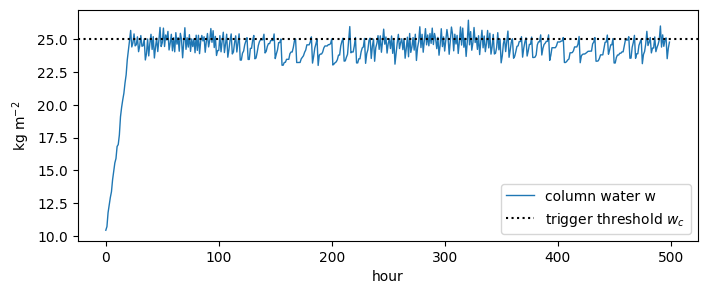
Now the failure at model scale. A single atmospheric column accumulates moisture from a prescribed, weather-like supply; when column water \(w\) exceeds a critical value \(w_c\), precipitation removes it at a fixed rate \(P_0\) — an on/off trigger of the kind convection schemes have used for decades. The scientific task: given observations of the column’s mean water content, calibrate \(w_c\).

DT_H = 1.0                       # time step, hours
N_STEPS = 2000
P0 = 2.0                         # precipitation rate when triggered, kg m^-2 per hour
key = jax.random.key(0)
supply = jnp.clip(0.5 * (1.0 + 0.8 * jnp.sin(2 * jnp.pi * jnp.arange(N_STEPS) / 240.0))
                  + 0.3 * jax.random.normal(key, (N_STEPS,)), 0.0, None)

def simulate(w_crit, precip):
    def one(w, E):
        P = precip(w, w_crit)
        w = jnp.clip(w + DT_H * (E - P), 0.0, None)
        return w, (w, P)
    _, (w, P) = jax.lax.scan(one, 10.0, supply)
    return w, P

hard_trigger = lambda w, w_crit: jnp.where(w > w_crit, P0, 0.0)

W_TRUE = 25.0
w_truth, P_truth = simulate(W_TRUE, hard_trigger)
OBS = float(jnp.mean(w_truth))
print(f"observed mean column water: {OBS:.2f} kg m^-2;  raining {float(jnp.mean(P_truth > 0)):.0%} of the time")

fig, ax = plt.subplots(figsize=(8, 3))
ax.plot(w_truth[:500], lw=1, label="column water w")
ax.axhline(W_TRUE, color="k", ls=":", label="trigger threshold $w_c$")
ax.set_xlabel("hour"); ax.set_ylabel("kg m$^{-2}$"); ax.legend()
plt.show()

observed mean column water: 24.43 kg m^-2;  raining 26% of the time

The failure: a loss that varies, and a gradient that is zero

The calibration loss clearly depends on \(w_c\) — and its derivative is identically zero. The trigger’s timing changes in discrete jumps as \(w_c\) varies, so the loss is a staircase: thousands of microscopic treads, each perfectly flat. Plotted at normal resolution it even looks smooth, which makes this failure mode treacherous — nothing warns you except the gradient’s suspicious exactness:

def loss_hard(w_crit):
    w, _ = simulate(w_crit, hard_trigger)
    return (jnp.mean(w) - OBS) ** 2

fig, (ax1, ax2) = plt.subplots(1, 2, figsize=(9, 3))
wc_wide = jnp.linspace(20.0, 30.0, 400)
ax1.plot(wc_wide, jax.vmap(loss_hard)(wc_wide))
ax1.set_xlabel("$w_c$"); ax1.set_ylabel("loss"); ax1.set_title("looks smooth...")
wc_zoom = jnp.linspace(24.99, 25.01, 400)
ax2.plot(wc_zoom, jax.vmap(loss_hard)(wc_zoom), lw=1)
ax2.set_xticks([24.99, 25.0, 25.01])
ax2.set_xlabel("$w_c$"); ax2.set_title("...is a staircase")
plt.tight_layout(); plt.show()

print("gradients:", [float(jax.grad(loss_hard)(wc)) for wc in [20.0, 23.0, 25.0, 27.0]])

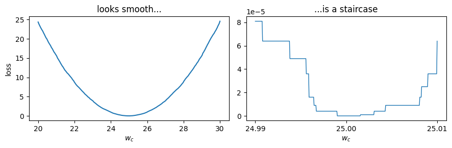
gradients: [0.0, 0.0, 0.0, 0.0]

Gradient descent receives zero at every point and goes nowhere. Note the contrast with Chapter 3.1: there the gradient was huge and meaningless; here it is zero and meaningless. Exact differentiation of the wrong microstructure produces both.

Fix 1: smooth the switch

Replace the on/off trigger with a sigmoid of width \(\delta\): precipitation ramps up smoothly around \(w_c\). The gradient immediately becomes informative — at the price of changed physics, and the price depends on \(\delta\) in both directions:

import optax

def calibrate(precip, w0=20.0, n=300, lr=0.2):
    wc, opt = jnp.array(w0), optax.adam(lr)
    state = opt.init(wc)
    def loss(w_crit):
        w, _ = simulate(w_crit, precip)
        return (jnp.mean(w) - OBS) ** 2
    step = jax.jit(jax.value_and_grad(loss))
    for _ in range(n):
        L, g = step(wc)
        updates, state = opt.update(g, state)
        wc = optax.apply_updates(wc, updates)
    return float(wc)

print("smoothing width   recovered w_c (truth 25.0)   drizzle below threshold")
for delta in [2.0, 0.5, 0.1]:
    smooth = lambda w, w_crit, d=delta: P0 * jax.nn.sigmoid((w - w_crit) / d)
    wc = calibrate(smooth)
    w, P = simulate(wc, lambda w_, c_: P0 * jax.nn.sigmoid((w_ - c_) / delta))
    drizzle = float(jnp.sum(jnp.where(w < wc, P, 0.0)) / jnp.sum(P))
    print(f"   {delta:4.1f}              {wc:6.2f}                     {drizzle:.0%} of total rain")

smoothing width   recovered w_c (truth 25.0)   drizzle below threshold

    2.0               26.89                     94% of total rain
    0.5               25.14                     83% of total rain

    0.1               28.79                     91% of total rain

The sweet spot is real but narrow. Too wide (\(\delta = 2\)): the model drizzles far from the threshold, its climate is biased, and the recovered \(w_c\) inherits the bias. Too narrow (\(\delta = 0.1\)): the sigmoid approaches the original staircase, the gradient signal collapses into spikes, and the optimizer strands far from truth. And at any width, the forward physics is altered — here a large share of rain falls in conditions where the true model produces none. Smoothing is a legitimate modeling decision (many modern schemes prefer smooth triggers on physical grounds); it is a poor afterthought.

Fix 2: reformulate the physics

Sometimes the discreteness is an implementation habit rather than a physical claim. A ramp trigger — precipitation proportional to the water excess, \(P = k\,\max(w - w_c,\, 0)\) — is as defensible physically, and its kink passes an informative (one-sided) gradient. Where a reformulation exists, it is the cleanest answer: the model you differentiate is the model you mean. The exercise below asks you to run it; the pattern to notice is that choosing differentiable physics up front beats repairing non-differentiable physics after the fact.

Fix 3: keep the physics, prescribe the derivative

When the hard switch is the model you mean, JAX allows a division of labor: the forward pass runs the exact discontinuous physics, and jax.custom_vjp substitutes a chosen derivative — here, the sigmoid’s — in the backward pass:

@jax.custom_vjp
def trigger(w, w_crit):
    return jnp.where(w > w_crit, P0, 0.0)          # exact forward physics

def trigger_fwd(w, w_crit):
    return trigger(w, w_crit), (w, w_crit)

def trigger_bwd(saved, dLdP):
    w, w_crit = saved
    s = jax.nn.sigmoid((w - w_crit) / 0.5)          # surrogate slope, width 0.5
    dP = P0 * s * (1 - s) / 0.5
    return (dLdP * dP, -dLdP * dP)

trigger.defvjp(trigger_fwd, trigger_bwd)

wc = calibrate(trigger)
print(f"custom_vjp calibration: recovered w_c = {wc:.3f}   (truth 25.0)")
w, P = simulate(wc, trigger)
print(f"forward physics exact: rain rate is only ever 0 or {P0}: "
      f"{bool(jnp.all((P == 0) | (P == P0)))}")

custom_vjp calibration: recovered w_c = 25.001   (truth 25.0)

forward physics exact: rain rate is only ever 0 or 2.0: True

Recovered to three decimal places, with the simulated physics bit-for-bit the hard trigger. The backward pass is now a lie — a deliberate, controlled one: the surrogate derivative says “moving \(w_c\) down makes rain more likely near the threshold,” which is true on average even though the pointwise derivative is zero. Machine learning knows this trick as the straight-through estimator, standard equipment for training through quantization and sampling [Blondel and Roulet, 2024]; the physical sciences increasingly use it for thresholds exactly like this one. Its limits: the surrogate’s bias is uncontrolled (no convergence theorem stands behind it), so the result deserves the verification habits of Chapter 3.5 — does the calibrated model match observations it was not trained on?

Three fixes, one decision rule: smooth if a smooth model is physically acceptable (and report the width as a model parameter); reformulate if the discreteness was never physical; surrogate-gradient if the discontinuous physics must stand. What is not on the menu is differentiating the hard switch and hoping — the zeros propagate silently into any larger model containing them.

Exercises.

1. Implement the ramp trigger \(P = 0.4\,\max(w - w_c, 0)\), generate its own truth, and calibrate. Why does even the one-sided kink gradient suffice here?

2. Vary the surrogate width in trigger_bwd over {0.1, 0.5, 2.0}. Which parts of the smoothing trade-off return, and which do not?

3. The ice line of Part 2 used tanh with a 2 K width — a Fix-1 choice made for you. Re-run Chapter 2.2’s calibration with width 0.2 K. What happens to the loss landscape and the descent?