3.5 Do you trust your gradient?

Part 3 has shown gradients that explode (3.1), exhaust memory (3.2), silently zero out (3.3), and detonate in the backward pass (3.4). The closing chapter turns those lessons into habits — the checks that separate the optimizer moved from the science is right. Three layers, in the order failures actually occur:

1. the gradient is numerically correct (it matches finite differences),

2. it is finite and well-scaled (no NaN, no precision rot),

3. it answers the question you meant to ask (the statistic, window, and ensemble are the ones your scientific claim is about).

None of these layers is expensive. All of them have caught real errors in real projects.

Learning goals

• Run finite-difference checks routinely, reading the step-size error curve correctly

• Know what single precision does to gradients — and to your ability to verify them

• Hunt NaNs with jax.debug_nans and jax.debug.print

• Apply a pre-publication checklist to any gradient-based result

import jax
import jax.numpy as jnp
import matplotlib.pyplot as plt

jax.config.update("jax_enable_x64", True)   # climate work needs double precision
# Running on Colab? First run:  %pip install -q optax equinox diffrax

Layer 1: the finite-difference check, done properly

The habit from Chapter 1.2, now with its full interpretation. The test model is the 0-D energy balance model of Chapter 1.3 (a 100-year rollout compressed into a loss); the check compares its autodiff gradient against central differences over a sweep of step sizes:

S0, SIGMA_SB = 1361.0, 5.67e-8

def make_loss(dtype):
    """Squared error of the 100-year EBM temperature vs a 290 K target."""
    def albedo(T):
        return 0.28 + 0.34 * 0.5 * (1.0 - jnp.tanh((T - 263.0) / 5.0))
    def loss(emissivity):
        def step(T, _):
            imbalance = S0 * (1 - albedo(T)) / 4 - emissivity * SIGMA_SB * T ** 4
            return T + jnp.asarray(86400.0 * 30 / 4e8, dtype) * imbalance, None
        T, _ = jax.lax.scan(step, jnp.asarray(288.0, dtype), None, length=1200)
        return (T - 290.0) ** 2
    return loss

loss64 = make_loss(jnp.float64)
g64 = jax.grad(loss64)(jnp.float64(0.61))

steps = jnp.logspace(-2, -11, 10)
def rel_error(loss_fn, g, x, dtype):
    errs = []
    for h in steps:
        hh = jnp.asarray(h, dtype)
        fd = (loss_fn(x + hh) - loss_fn(x - hh)) / (2 * hh)
        errs.append(abs(float((fd - g) / g)))
    return errs

err64 = rel_error(loss64, g64, jnp.float64(0.61), jnp.float64)
plt.loglog(steps, err64, "o-")
plt.gca().invert_xaxis()
plt.xlabel("finite-difference step h"); plt.ylabel("relative error vs autodiff")
plt.title("The V curve: truncation error (left) meets roundoff (right)")
plt.show()
print(f"best agreement: {min(err64):.1e} at h = {float(steps[err64.index(min(err64))]):.0e}")

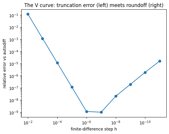
best agreement: 9.8e-10 at h = 1e-07

Read the V shape, not just its bottom. The left slope is the finite difference’s truncation error (\(O(h^2)\) for central differences — the check’s own inaccuracy, not autodiff’s); the right slope is floating-point cancellation. A healthy check bottoms out near \(10^{-9}\)–\(10^{-11}\) in double precision. Three verdicts are possible: a clean V touching ~\(10^{-10}\) (gradient verified); a V bottoming at ~\(10^{-3}\) (suspect the loss — noise, a hidden discontinuity, single precision); no V at all, errors of order one (the gradient is simply wrong — often a stop_gradient or a non-differentiable operation upstream). For multi-dimensional inputs, check a few random directional derivatives rather than every component.

Layer 2: precision

JAX defaults to single precision — a deep-learning inheritance that climate work must override (every notebook in this book enables jax_enable_x64 in its first cell). The same model in float32 shows both symptoms: the gradient itself drifts (roundoff accumulated across 1,200 steps contaminates the backward pass), and the finite-difference check loses its floor, so the drift cannot even be diagnosed cleanly:

loss32 = make_loss(jnp.float32)
g32 = jax.grad(loss32)(jnp.float32(0.61))
print(f"float64 gradient: {float(g64):+.5f}")
print(f"float32 gradient: {float(g32):+.5f}   ({abs(float((g32-g64)/g64)):.1%} off)")

err32 = rel_error(loss32, g32, jnp.float32(0.61), jnp.float32)
plt.loglog(steps, err64, "o-", label="float64")
plt.loglog(steps, err32, "s-", label="float32")
plt.gca().invert_xaxis()
plt.xlabel("step h"); plt.ylabel("relative error"); plt.legend()
plt.title("float32: the check bottoms out three orders of magnitude early")
plt.show()

float64 gradient: -24.69132
float32 gradient: -24.52714   (0.7% off)

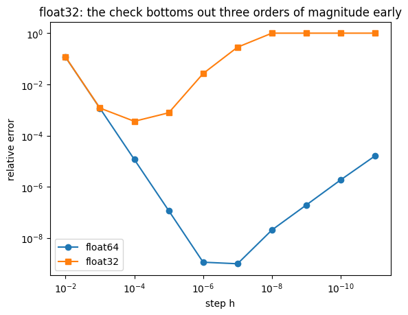
A 0.7% gradient error and a verification floor of \(10^{-4}\). Where the line sits in practice: neural-network weights tolerate single precision well (deep learning runs on it), but physical state carried across many time steps — budgets, conserved quantities, anything whose gradient you intend to verify — wants float64. Mixed precision is a performance tool for Part-4-scale work; adopt it after the double-precision version passes its checks, never before.

Layer 3 (mechanics): hunting NaNs

A NaN in the gradient usually enters at one operation and floods everything downstream, so the tool that matters is the one that catches the birth. JAX’s debug mode re-runs the offending computation un-jitted and raises at the first NaN:

def suspicious(x):
    return jnp.where(x > 0.0, jnp.sqrt(x), 0.0)     # Chapter 3.3's trap

jax.config.update("jax_debug_nans", True)
try:
    jax.grad(suspicious)(0.0)
except FloatingPointError as e:
    print("caught at birth:", str(e).splitlines()[0])
finally:
    jax.config.update("jax_debug_nans", False)

fixed = lambda x: jnp.where(x > 0.0, jnp.sqrt(jnp.where(x > 0.0, x, 1.0)), 0.0)
print("after the double-where fix:", jax.grad(fixed)(0.0))

Invalid nan value encountered in the backward pass of a jax.jit function. Calling the de-optimized backward pass.
caught at birth: invalid value (nan) encountered in mul
after the double-where fix: 0.0

The usual suspects, in rough order of frequency: sqrt/log/fractional powers evaluated at zero (often inside a where whose untaken branch still gets differentiated — the double-where idiom is the fix); divisions with denominators that a trajectory can drive to zero; and exponential overflow in the backward pass of an unstable rollout (in which case the NaN is a symptom, and Chapters 3.1/3.4 are the disease). For inspecting values inside jitted code without leaving compiled execution, jax.debug.print("{x}", x=...) prints at runtime — the tracing-safe replacement for print from Chapter 1.1.

Layer 3 (science): is it the right gradient?

The final layer has no tool, only a question: of what, exactly, is this the derivative? Chapter 3.1 in one picture — the same model, the same parameter, two different questions:

K = 40
def l96_step(u, F):
    def f(u):
        return (jnp.roll(u, -1) - jnp.roll(u, 2)) * jnp.roll(u, 1) - u + F
    k1 = f(u); k2 = f(u + 0.005 * k1); k3 = f(u + 0.005 * k2); k4 = f(u + 0.01 * k3)
    return u + 0.01 / 6 * (k1 + 2 * k2 + 2 * k3 + k4)

u0 = 8.0 + 0.5 * jax.random.normal(jax.random.key(0), (K,))
u_spun, _ = jax.lax.scan(lambda u, _: (l96_step(u, 8.0),) * 2, u0, None, length=2000)

def misfit(F, n_steps):
    _, traj = jax.lax.scan(lambda u, _: (l96_step(u, F),) * 2, u_spun, None, length=n_steps)
    return jnp.mean((traj - 2.34) ** 2)             # vs the F=8 climate mean

Fs = jnp.linspace(7.5, 8.5, 121)
fig, (ax1, ax2) = plt.subplots(1, 2, figsize=(9, 3))
ax1.plot(Fs, jax.vmap(lambda F: misfit(F, 50))(Fs))
ax1.set_title("window 0.5: weather question,\nusable gradient")
ax2.plot(Fs, jax.vmap(lambda F: misfit(F, 1600))(Fs))
ax2.set_title("window 16: climate question,\ngradient of the noise")
for ax in (ax1, ax2): ax.set_xlabel("F")
plt.tight_layout(); plt.show()

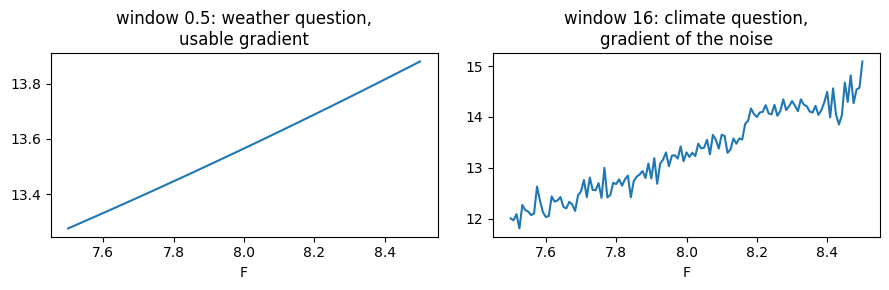
If a reviewer asked “what is the derivative in your figure of?”, the left panel has an answer (“the 0.5-unit trajectory misfit, which is smooth in F”) and the right panel does not. Making the window, statistic, and ensemble explicit parts of the claim — and showing the result is robust to reasonable changes in them — is what distinguishes a gradient-based result from a gradient-shaped artifact.

The checklist

Before believing any gradient-based result

1. Finite-difference check passes — a clean V bottoming near 1e-9 in float64, re-run whenever the model changes.

2. No NaN/Inf anywhere in the loss or gradient over the whole parameter range explored (jax_debug_nans during development).

3. Precision is sufficient: float64 for verification; any reduced-precision run agrees with the float64 reference on a spot check.

4. The loss is smooth at the scale the optimizer moves — zoom in (Chapters 3.1, 3.3); thresholds smoothed or surrogated deliberately, with the choice reported.

5. The statistic matches the claim: window length, averaging, and ensemble are stated, and the conclusion survives doubling the window / changing the seed.

6. Optimization end-state is defensible: loss at the expected floor (Chapter 2.2), parameters physical, and the result reproduced from a second starting point.

Where to next

The tools in this book — grad through scan, checkpointing, implicit differentiation, surrogate gradients, truncated estimators — are the same ones running inside the current generation of differentiable Earth-system efforts, from JAX-native dynamical cores to hybrid models trained through their solvers [Gelbrecht et al., 2023, Kochkov et al., 2024, Shen et al., 2023]. The gap between this book’s 60-point toys and those systems is engineering (Part 4, when we write it), not concept. The concepts — and their failure modes — you now own.

Exercises.

1. Break the Chapter 2.2 calibration deliberately: insert a stop_gradient somewhere in the model and confirm the finite-difference check catches it (and note which verdict it produces).

2. Add jax.debug.print to the 0-D EBM step to watch the temperature during a diverging integration (take dt 100× larger). Where does the NaN first appear?

3. Take any result you produced in Part 2 and run it through the checklist. Write down which items you had silently skipped.