3.2 Memory and the cost of long simulations

3.2 Memory and the cost of long simulations#

Reverse-mode differentiation requires running the chain rule backward, it must revisit the forward computation in reverse order, which means the intermediate states of the entire integration must be available, stored or recomputed. A simulation that runs comfortably forward can therefore be undifferentiable in practice: the forward model needs memory for one time step; its adjoint, naively, for all of them.

For the 60-point model used here this costs megabytes and is invisible. For an atmosphere at kilometer resolution it is the difference between feasible and not. This chapter measures the scaling, applies the standard cure — checkpointing, the compute-for-memory trade formalized by Griewank [Griewank and Walther, 2008] — and ends with the elegant special case where the whole problem disappears: differentiating a steady state.

import jax
import jax.numpy as jnp
import matplotlib.pyplot as plt

jax.config.update("jax_enable_x64", True)   # climate work needs double precision
# Running on Colab? First run:  %pip install -q optax equinox diffrax

Measuring the memory#

JAX can report the temporary memory a compiled function will allocate, before running it. The function below builds a differentiated simulation of the Budyko–Sellers model (the Part 2 model, redefined in the cell above) in three variants and asks the compiler for its scratch-space budget:

def rollout_loss(n_steps, variant="plain"):
    """Mean-square final temperature after n_steps, as a function of diffusivity."""
    def loss(D):
        p = dict(default_params, D=D)
        step = lambda T: T + dt / heat_capacity * energy_tendency(T, p)
        if variant == "remat":
            step = jax.checkpoint(step)
        if variant == "chunked":
            chunk = int(n_steps ** 0.5)
            @jax.checkpoint
            def inner(T):
                T, _ = jax.lax.scan(lambda t, _: (step(t), None), T, None, length=chunk)
                return T
            T, _ = jax.lax.scan(lambda t, _: (inner(t), None), T_start, None,
                                length=n_steps // chunk)
        else:
            T, _ = jax.lax.scan(lambda t, _: (step(t), None), T_start, None, length=n_steps)
        return jnp.mean(T ** 2)
    return loss

def temp_memory_mb(fn):
    compiled = jax.jit(fn).lower(jnp.float64(0.48)).compile()
    return compiled.memory_analysis().temp_size_in_bytes / 1e6

steps = [1000, 4000, 16000, 64000]
table = {v: [temp_memory_mb(jax.grad(rollout_loss(n, v))) for n in steps]
         for v in ["plain", "remat", "chunked"]}
fwd = [temp_memory_mb(rollout_loss(n)) for n in steps]

print("steps     forward   grad      grad+remat  grad+chunked")
for i, n in enumerate(steps):
    print(f"{n:6d}   {fwd[i]:7.3f}   {table['plain'][i]:7.2f}   {table['remat'][i]:9.2f}"
          f"   {table['chunked'][i]:9.3f}   MB")

plt.loglog(steps, table["plain"], "o-", label="grad (stores every step)")
plt.loglog(steps, table["remat"], "s-", label="grad + per-step remat")
plt.loglog(steps, table["chunked"], "d-", label="grad + two-level checkpointing")
plt.loglog(steps, fwd, "k^-", label="forward only")
plt.xlabel("simulation length (steps)"); plt.ylabel("temporary memory (MB)")
plt.legend(); plt.title("Adjoint memory vs simulation length")
plt.show()

steps     forward   grad      grad+remat  grad+chunked
   0.002      1.43        0.48       0.064   MB
   0.002      5.73        1.92       0.125   MB
   0.002     22.91        7.68       0.245   MB
   0.002     91.65       30.72       0.487   MB

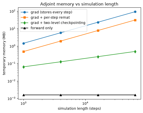
../_images/91366b705fccca731ee2d7f786ea99856d297414bebe0aa5d9d1868fe9f8608a.png

Four regimes, one story:

Forward only is flat: a time-stepper needs the current state and nothing else.
Plain grad grows linearly — every step’s state is saved for the backward pass. Sixty-four thousand steps of this toy already book ~90 MB; scale the state by the size of a GCM field and limitations arise quickly.
Per-step rematerialization (jax.checkpoint on the step function) tells JAX to discard each step’s internal intermediates and recompute them during the backward pass. It cuts the constant (~3× here) but not the slope: the per-step states themselves must still be kept.
Two-level checkpointing changes the slope. Split \(N\) steps into \(\sqrt{N}\) chunks of \(\sqrt{N}\): store only chunk boundaries, and recompute inside one chunk at a time during the backward sweep. Memory drops to \(O(\sqrt{N})\) — a 188× saving at 64,000 steps — for roughly one extra forward pass of compute. Recursive (binomial) schedules push this to logarithmic memory; diffrax (Chapter 3.4) implements them for you.

The knob to remember: jax.checkpoint placed around a scan body controls what is stored across the loop, and nesting scans sets the storage granularity.

Steady states: sidestep the trajectory entirely#

When the quantity of interest is an equilibrium, the trajectory that reached it is scaffolding — and there is a way to differentiate that never stores it. At a steady state, the energy tendency vanishes: \(\mathcal{F}(T^{*}, \theta) = 0\). Differentiating this identity (the implicit function theorem) gives the sensitivity of the equilibrium directly:

\[ \frac{\partial T^{*}}{\partial \theta} = -\left(\frac{\partial \mathcal{F}}{\partial T}\right)^{-1} \frac{\partial \mathcal{F}}{\partial \theta}, \]

one linear solve against the Jacobian at the equilibrium, however long the spin-up took. In JAX this is expressed by attaching a custom derivative rule to the spin-up function — forward pass unchanged, backward pass replaced by the linear solve:

@jax.custom_vjp
def equilibrium(D):
    return integrate(T_start, dict(default_params, D=D), n_years=60)

def equilibrium_fwd(D):
    T_eq = equilibrium(D)
    return T_eq, (T_eq, D)

def equilibrium_bwd(saved, dLdT):
    T_eq, D = saved
    residual = lambda T, D: energy_tendency(T, dict(default_params, D=D))
    dF_dT = jax.jacobian(residual, argnums=0)(T_eq, D)      # 60x60 Jacobian
    dF_dD = jax.jacobian(residual, argnums=1)(T_eq, D)
    adjoint = jnp.linalg.solve(dF_dT.T, dLdT)               # one linear solve
    return (-adjoint @ dF_dD,)

equilibrium.defvjp(equilibrium_fwd, equilibrium_bwd)

g_implicit = jax.grad(lambda D: jnp.mean(equilibrium(D)))(0.48)
g_unrolled = jax.grad(lambda D: jnp.mean(integrate(T_start,
                      dict(default_params, D=0.0 + D), n_years=60)))(0.48)
print(f"d(global-mean T_eq)/dD   implicit: {float(g_implicit):.6f}")
print(f"d(global-mean T_eq)/dD   unrolled: {float(g_unrolled):.6f}")

d(global-mean T_eq)/dD   implicit: 61.652069
d(global-mean T_eq)/dD   unrolled: 61.652065

The two agree to seven digits — but the implicit version’s backward pass is one 60×60 linear solve, independent of whether the spin-up took 60 years or 60,000. The same idea, packaged, appears as jax.lax.custom_root and as the optimistix/ diffrax libraries’ implicit differentiation of solvers and root-finders (Chapter 3.4). It applies whenever the output satisfies an equation — equilibria, implicit time steps, optimization inner loops — and it is the cleanest large-scale memory fix available: no trajectory, no checkpoints, exact gradient.

Two caveats for practice. The equilibrium must actually be reached (the identity differentiated is \(\mathcal{F}=0\); a half-spun-up state gives a subtly wrong gradient), and for large states the explicit Jacobian is replaced by matrix-free linear solves — the mathematics is unchanged.

Exercises.

At 64,000 steps, time (rather than measure memory for) the plain and chunked gradients. How much compute did the 188× memory saving cost?
Implement three-level checkpointing (nest one more scan). Predict the memory scaling before you measure it.
The implicit gradient needs \(\partial\mathcal{F}/\partial T\) to be invertible. What does a singular Jacobian mean physically? (Chapter 1.3’s fold is the answer.)

3.2 Memory and the cost of long simulations

Contents

3.2 Memory and the cost of long simulations#

Measuring the memory#

Steady states: sidestep the trajectory entirely#