
2.4 Hybrid physics–ML modeling#
The diffusion term in Budyko–Sellers is a closure: it stands in for the poleward energy transport of weather systems the model does not resolve, compressing all of storm-track dynamics into one coefficient. Replacing closures with ones learned from data is the central promise of machine learning for climate modeling.
This chapter builds a true model whose transport the coarse model misrepresents, inserts a small neural network as a transport correction, and trains it two ways:
Offline (a priori): fit the network to diagnosed transport values, by ordinary supervised regression. Requires knowing the true fluxes — data that in reality only a field campaign or a high-resolution simulation can provide.
Online (a posteriori): run the hybrid model, compare its climate to observations, and differentiate the misfit through the entire simulation back to the network weights [Frezat et al., 2022, Kochkov et al., 2021]. Requires only observable outputs — but requires the model to be differentiable.
import jax
import jax.numpy as jnp
import matplotlib.pyplot as plt

jax.config.update("jax_enable_x64", True)   # climate work needs double precision
# Running on Colab? First run:  %pip install -q optax equinox diffrax
A “true” model with structure the coarse model lacks#
In the “true” model, diffusivity peaks in the mid-latitude storm tracks at nearly twice the background value. The coarse model keeps diffusivity constant, this is a structural error no constant-\(D\) calibration can remove. The generalized integrator below accepts a per-edge diffusivity and an optional extra flux (the future neural network’s slot):
lat_edge = jnp.rad2deg(jnp.arcsin(x_edge[1:-1]))
D_truth = 0.48 * (1.0 + 0.9 * jnp.exp(-(((jnp.abs(lat_edge) - 45.0) / 15.0) ** 2)))

def integrate2(T0, D_edge, extra_flux=None, n_years=30):
    """Budyko-Sellers with per-edge diffusivity and an optional learned flux."""
    def tendency(T):
        absorbed = Q * s_x * (1.0 - albedo(T, default_params))
        emitted = A_olr + B_olr * T
        flux = D_edge * (1.0 - x_edge[1:-1] ** 2) * jnp.diff(T) / dx
        if extra_flux is not None:
            flux = flux + extra_flux(T)
        flux = jnp.concatenate([jnp.zeros(1), flux, jnp.zeros(1)])
        return absorbed - emitted + jnp.diff(flux) / dx
    def step(T, _):
        return T + dt / heat_capacity * tendency(T), T
    T_final, traj = jax.lax.scan(step, T0, None, length=int(n_years * 365.25 * 86400 / dt))
    return T_final, traj

T_truth, truth_traj = integrate2(T_start, D_truth)
T_coarse, _ = integrate2(T_start, 0.48)
rmse = lambda a, b: float(jnp.sqrt(jnp.mean((a - b) ** 2)))
print(f"coarse-model climate error: {rmse(T_coarse, T_truth):.2f} K RMSE")

plt.plot(lat, T_truth, "k", lw=2, label="truth (structured transport)")
plt.plot(lat, T_coarse, "C3", lw=2, label="coarse model (constant D)")
plt.xlabel("latitude (deg)"); plt.ylabel("temperature (degC)"); plt.legend()
plt.title("A 4.5 K structural bias, concentrated at high latitudes")
plt.show()
coarse-model climate error: 4.49 K RMSE
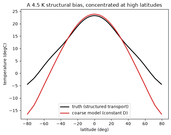
The extra mid-latitude transport in the “true model” carries enough heat poleward to melt the ice caps; the coarse model, missing it, keeps them, a nearly 20 K polar error and a qualitatively different climate. This is the kind of bias a learned closure should fix.
The closure#
A three-layer perceptron maps local conditions at each cell edge — temperature, temperature gradient, and position — to a flux correction. Locality is a physical choice (transport closures should not act at a distance), and the \((1-x^2)\) factor guarantees no flux through the poles. Note what the network is not told: the shape of \(D_\mathrm{truth}\).
import equinox as eqx
import optax

def edge_features(T):
    T_edge = 0.5 * (T[:-1] + T[1:])
    grad_T = jnp.diff(T) / dx
    return jnp.stack([T_edge / 30.0, grad_T / 100.0, x_edge[1:-1]], axis=-1)

class TransportClosure(eqx.Module):
    mlp: eqx.nn.MLP
    def __init__(self, key):
        self.mlp = eqx.nn.MLP(in_size=3, out_size=1, width_size=32, depth=2, key=key)
    def __call__(self, T):
        raw = jax.vmap(self.mlp)(edge_features(T))[:, 0]
        return 50.0 * (1.0 - x_edge[1:-1] ** 2) * raw     # W m^-2 scale

closure0 = TransportClosure(jax.random.key(2))
n_weights = sum(a.size for a in jax.tree.leaves(eqx.filter(closure0, eqx.is_array)))
print(f"closure parameters: {n_weights}")
closure parameters: 1217
Offline training: regression on diagnosed fluxes#
Pretend a high-resolution campaign has measured the transport the coarse model misses, at snapshots along the truth’s evolution. Supervised learning on those diagnosed fluxes is standard regression — no differentiable model required:
snapshots = truth_traj[jnp.arange(200, 40000, 200)]        # 199 states along the spin-up

def missing_flux(T):
    return (D_truth - 0.48) * (1.0 - x_edge[1:-1] ** 2) * jnp.diff(T) / dx

flux_targets = jax.vmap(missing_flux)(snapshots)

def train(model, loss_fn, learning_rate, n_iters):
    opt = optax.adam(learning_rate)
    opt_state = opt.init(eqx.filter(model, eqx.is_array))
    @eqx.filter_jit
    def one(model, opt_state):
        L, g = eqx.filter_value_and_grad(loss_fn)(model)
        updates, opt_state = opt.update(g, opt_state)
        return eqx.apply_updates(model, updates), opt_state, L
    for i in range(n_iters):
        model, opt_state, L = one(model, opt_state)
    return model, float(L)

def offline_loss(model):
    return jnp.mean((jax.vmap(model)(snapshots) - flux_targets) ** 2)

closure_offline, L = train(closure0, offline_loss, 3e-3, 1500)
print(f"offline: final flux-fitting loss {L:.4f} (W m^-2)^2")
offline: final flux-fitting loss 0.0065 (W m^-2)^2
Online training: through the solver#
Now suppose no flux measurements exist, only the observable climate (the equilibrium
temperature profile). The online loss runs the hybrid model for twelve years and
compares its output to the truth’s climate; grad carries the misfit backward through
every time step to the network weights. Two variants: one trained on the full profile,
one on only the five observed latitudes of Chapter 2.3.
T_coarse_eq, _ = integrate2(T_start, 0.48)      # warm start for training rollouts

def online_loss(model):
    T_final, _ = integrate2(T_coarse_eq, 0.48, extra_flux=model, n_years=12)
    return jnp.mean((T_final - T_truth) ** 2)

obs_idx = jnp.array([jnp.argmin(jnp.abs(lat - l)) for l in [-60.0, -30.0, 0.0, 30.0, 60.0]])
def online_sparse_loss(model):
    T_final, _ = integrate2(T_coarse_eq, 0.48, extra_flux=model, n_years=12)
    return jnp.mean((T_final[obs_idx] - T_truth[obs_idx]) ** 2)

schedule = optax.exponential_decay(3e-3, transition_steps=150, decay_rate=0.5)
closure_online, L1 = train(closure0, online_loss, schedule, 500)
closure_sparse, L2 = train(closure0, online_sparse_loss, schedule, 500)
print(f"online (full profile): final loss {L1:.4f} K^2")
print(f"online (5 latitudes):  final loss {L2:.4f} K^2")
online (full profile): final loss 0.1171 K^2
online (5 latitudes):  final loss 0.0067 K^2
The comparison#
Each closure now runs inside the coarse model from the original cold start, for 40 years, longer than any training rollout, from a state none of them saw:
results = {}
for name, m in [("offline (flux data)", closure_offline),
                ("online (full profile)", closure_online),
                ("online (5 latitudes)", closure_sparse)]:
    T_final, _ = integrate2(T_start, 0.48, extra_flux=m, n_years=40)
    results[name] = T_final
    print(f"{name:24s} climate RMSE vs truth: {rmse(T_final, T_truth):6.3f} K")
print(f"{'no closure':24s} climate RMSE vs truth: {rmse(T_coarse, T_truth):6.3f} K")

plt.plot(lat, T_truth, "k", lw=2.5, label="truth")
plt.plot(lat, T_coarse, "C3", ls="--", label="coarse, no closure")
for (name, T_f), c in zip(results.items(), ["C0", "C1", "C2"]):
    plt.plot(lat, T_f, c, lw=1.5, label=name)
plt.xlabel("latitude (deg)"); plt.ylabel("temperature (degC)")
plt.legend(fontsize=8); plt.title("Hybrid climates vs truth")
plt.show()
offline (flux data)      climate RMSE vs truth:  0.016 K
online (full profile)    climate RMSE vs truth:  0.342 K
online (5 latitudes)     climate RMSE vs truth:  0.643 K
no closure               climate RMSE vs truth:  4.494 K
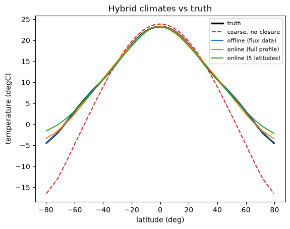
All three hybrids remove nearly all of the 4.5 K structural bias. Reading the table with the data requirements in mind:
Offline is excellent here, when its data exist. The diagnosed-flux dataset determines the closure almost completely, and the model’s strong damping keeps small flux errors from compounding. The result would look very different in a model where errors grow: in turbulence, offline-trained closures are notorious for drifting or destabilizing when coupled, precisely because a-priori skill does not measure the coupled feedback loop [Frezat et al., 2022]. Part 3.1 introduces the error-growth regime where that distinction bites.
Online needs only what is observable. Within half a kelvin of truth using nothing but the equilibrium temperature profile and within a kelvin using five numbers per observation time. No flux was ever measured. This is the regime real Earth-system closure learning lives in, and it is unavailable without a differentiable model: the gradient of the 12-year climate with respect to each of the 1,000+ network weights is what
graddelivered through the solver.The two can be combined. offline pre-training followed by online fine-tuning may inherit the best of both.
Exercises.
Give the offline network a fraction of the snapshots (every 2,000th step). How does its coupled RMSE degrade compared to the online closures?
The online closures were never told to conserve energy. Check: integrate each learned flux’s divergence over the globe. How large is the spurious source, and how would you constrain it to zero by construction?
Train the sparse-online closure with observations at 2 latitudes instead of 5. Where does the hybrid climate degrade first?